Buffer Operations

Create buffers around geometries and use them for proximity analysis in the FILTERING tab.

Overview

A buffer is a polygon representing all points within a specified distance from a geometry. In FilterMate, buffers are configured in the FILTERING tab alongside geometric predicates for proximity-based spatial filtering.

Key Uses

Buffers are essential for:

Proximity analysis - Find features near something (e.g., buildings within 200m of roads)
Impact zones - Define areas of influence (e.g., noise buffer around airport)
Service areas - Coverage analysis (e.g., 500m walking distance to transit)
Safety zones - Exclusion boundaries (e.g., 100m buffer around hazards)

Location in Interface

Buffer configuration is in the FILTERING tab, below the geometric predicates selector. Buffers are applied to the reference layer geometry before spatial comparison.

Key Concepts

Distance: How far the buffer extends (in specified units)
Unit: Distance measurement (meters, kilometers, feet, miles, degrees)
Buffer Type: Algorithm used (Standard, Fast, or Segment)
Integration: Buffers work with spatial predicates (Intersects, Contains, etc.)

Buffer Types

FilterMate supports three buffer algorithms in the FILTERING tab, each with different performance and accuracy characteristics.

1. Standard Buffer (Default)

The standard algorithm creates accurate buffers suitable for most use cases.

Characteristics:

✅ Accurate results
✅ Handles complex geometries well
✅ Good for most use cases
⚠️ Moderate performance on large datasets

When to Use:

General proximity analysis
Planning applications
Regulatory compliance (accuracy required)
Medium-sized datasets (<10k features)

Example Configuration:

FILTERING Tab:
- Buffer Distance: 500
- Buffer Unit: meters
- Buffer Type: Standard
- Segments: 16 (smooth curves)

2. Fast Buffer

The fast algorithm prioritizes performance over precision.

Characteristics:

⚡ 2-5x faster than standard
⚠️ Lower geometric accuracy
✅ Good for large datasets
✅ Suitable for visualization and exploration

When to Use:

Large datasets (>50k features)
Interactive exploration in QGIS
Approximate analysis where precision isn't critical
Quick visualization of proximity zones

Performance Comparison:

Dataset Size  | Standard | Fast  | Speed Gain
--------------|----------|-------|------------
1,000 features| 0.5s     | 0.2s  | 2.5x
10,000        | 4.2s     | 1.1s  | 3.8x
50,000        | 21.3s    | 5.8s  | 3.7x
100,000       | 45.1s    | 11.2s | 4.0x

Example Configuration:

FILTERING Tab:
- Buffer Distance: 1000
- Buffer Unit: meters
- Buffer Type: Fast
- Fewer segments for speed

3. Segment Buffer

The segment buffer creates buffers with customizable segmentation for fine control over smoothness vs performance.

Characteristics:

✅ Fine control over segment count
✅ Balance accuracy vs speed
✅ Good for publication-quality outputs
⚠️ Requires understanding of trade-offs

When to Use:

Publication-quality maps
When you need specific smoothness
Custom performance tuning
Advanced users wanting control

Segment Count Guidelines:

4-8 segments: Fast, angular appearance
16 segments: Balanced (default)
32-64 segments: Smooth curves, slower
64+ segments: Publication quality, slowest

Example Configuration:

FILTERING Tab:
- Buffer Distance: 200
- Buffer Unit: meters
- Buffer Type: Segment
- Segments: 32 (high quality)

Buffer Configuration in FILTERING Tab

Distance and Unit Selection

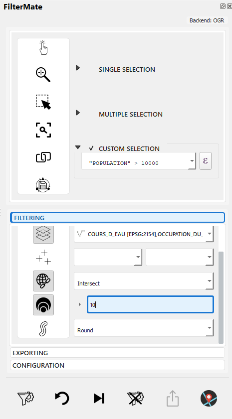
Configure buffer distance and select unit

Supported Units:

Meters (m) - Most common for projected CRS
Kilometers (km)
Feet (ft) - US State Plane
Miles (mi)
Degrees - Geographic CRS (use with caution)

CRS Matters

Ensure your layer uses an appropriate CRS:

Projected (meters, feet): UTM, State Plane, local projections → Use meters/feet
Geographic (degrees): WGS84, NAD83 → Convert to projected CRS first for accurate buffers

Distance Examples:

Urban planning:    50-500m
Transit access:    400-800m (walking distance)
Noise zones:       1-5km
Environmental:     100m-10km
Regional analysis: 10-100km

Buffer Type Selection

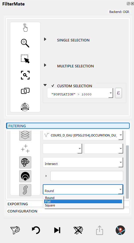
Choose buffer algorithm: Standard, Fast, or Segment

Selection Criteria:

Scenario	Recommended Type	Why
Quick exploration	Fast	Speed over precision
Official reporting	Standard	Good accuracy
Large datasets (&>;50k)	Fast	Performance
Publication maps	Segment (32+)	Visual quality
Regulatory compliance	Standard	Reliable accuracy

Buffer Integration with Geometric Filtering

Buffers work seamlessly with spatial predicates in the FILTERING tab:

Workflow:

Select source layer (e.g., "buildings")
Select spatial predicate (e.g., "Intersects")
Select reference layer (e.g., "roads")
Configure buffer: 200m, Standard type
Click FILTER

What Happens:

Reference layer geometry is buffered by 200m
Spatial predicate (Intersects) is applied between source layer and buffered reference
Result: Buildings that intersect roads within 200m

Example Use Cases:

Source Layer	Predicate	Reference Layer	Buffer	Result
Buildings	Intersects	Roads	200m	Buildings within 200m of roads
Parcels	Within	Protected Zone	50m	Parcels within 50m inside zone
Facilities	Disjoint	Hazards	500m	Facilities >500m` from hazards
POIs	Contains	District + Buffer	100m	POIs in district + 100m margin
else OGR Fallback
Q->>Q: QGIS buffer processing
Q->>Q: Generate buffers
end

Q->>FM: Buffer count + preview FM->>U: Display result (1,234 features)

U->>FM: Apply buffer filter FM->>Q: Apply spatial filter Q->>U: Show filtered map

## Practical Examples

### Urban Planning

#### Transit Coverage Analysis
```python
# 400m walk to transit stations
buffer_type = "standard"
distance = 400
segments = 16

# Find residential areas NOT covered
expression = """
NOT within(
    $geometry,
    buffer(
        geometry(get_feature('transit_stations', 'active', 'yes')),
        400
    )
)
AND land_use = 'residential'
"""

Noise Impact Zones

# Highway noise zones (tiered)
# 100m: High impact
# 300m: Moderate impact
# 500m: Low impact

# High impact properties
expression = """
intersects(
    $geometry,
    buffer(geometry(get_feature('highways', 'type', 'major')), 100)
)
AND property_type = 'residential'
"""

Environmental Analysis

Riparian Buffer Protection

# 30m protected buffer around streams
buffer_type = "standard"
distance = 30
segments = 16

expression = """
intersects(
    $geometry,
    buffer(geometry(get_feature('streams', 'class', 'perennial')), 30)
)
AND development_status = 'proposed'
"""

Wildlife Corridor Analysis

# 500m habitat buffer
buffer_type = "geodesic"  # Large area, accurate
distance = 500
segments = 32

expression = """
within(
    $geometry,
    buffer(geometry(get_feature('habitats', 'priority', 'high')), 500)
)
AND land_cover = 'forest'
"""

Emergency Services

Fire Station Coverage

# 5km service area (quick response)
buffer_type = "fast"  # Large dataset
distance = 5000
segments = 8

expression = """
NOT within(
    centroid($geometry),
    buffer(
        aggregate('fire_stations', 'collect', $geometry),
        5000
    )
)
AND zone_type = 'residential'
"""

Evacuation Zone

# 2km evacuation buffer around hazard
buffer_type = "geodesic"
distance = 2000
segments = 32

expression = """
intersects(
    $geometry,
    buffer(geometry(get_feature('hazards', 'status', 'active')), 2000)
)
"""

Buffer + Filter Combinations

Multiple Buffer Zones

-- Properties in different risk zones
CASE
    WHEN distance($geometry, @hazard_geom) < 100 THEN 'high_risk'
    WHEN distance($geometry, @hazard_geom) < 500 THEN 'medium_risk'
    WHEN distance($geometry, @hazard_geom) < 1000 THEN 'low_risk'
    ELSE 'safe'
END = 'high_risk'

Exclusion Zones

-- Available land (not in protected buffer)
land_use = 'undeveloped'
AND disjoint(
    $geometry,
    buffer(geometry(get_feature('protected', 'status', 'active')), 500)
)
AND area($geometry) > 10000

Proximity to Multiple Features

-- Near transit OR major roads
(
    distance($geometry, geometry(get_feature('transit', 'type', 'station'))) < 400
    OR
    distance($geometry, geometry(get_feature('roads', 'class', 'highway'))) < 200
)
AND zone = 'commercial'

Performance Optimization

Backend Comparison

Backend	Standard	Fast	Geodesic
PostgreSQL	⚡⚡⚡ Fast	⚡⚡⚡⚡ Faster	⚡⚡ Moderate
Spatialite	⚡⚡ Moderate	⚡⚡⚡ Fast	⚡ Slow
OGR	⚡ Slow	⚡⚡ Moderate	❌ N/A

Tips for Large Datasets

Use Fast Buffer for Exploration

# Quick interactive analysis
buffer_type = "fast"
segments = 8

Switch to Standard for Final Results

# Accurate final analysis
buffer_type = "standard"
segments = 16

Reduce Segments

# Balance accuracy and speed
segments = 8  # Instead of 32

Use PostgreSQL Backend
- Hardware-accelerated buffering
- Spatial index support
- 3-5x faster than Spatialite

Memory Considerations

# For 100k features with 500m buffers:
# - Fast buffer: ~200 MB RAM
# - Standard buffer: ~500 MB RAM
# - Geodesic buffer: ~800 MB RAM

Backend-Specific Behavior

PostgreSQL

Complete Buffer Workflow Example

Scenario: Find all buildings within 200m of roads

This example shows how buffers integrate with geometric filtering in the FILTERING tab.

Step-by-Step:

1. Open FILTERING tab

2. Select "buildings" as source layer

3. Select "Intersects" spatial predicate

4. Select "roads" as reference layer

5. Set buffer distance: 200, unit: meters

6. Select buffer type: Standard

7. Verify indicators: has_geometric_predicates, has_buffer_value, has_buffer_type all active

8. Click FILTER button

9. Progress bar shows processing (backend: PostgreSQL or Spatialite)

10. Results: 3,847 buildings within 200m of roads displayed on map

What Happened Behind the Scenes:

Roads layer geometry was buffered by 200m using Standard algorithm
Intersects predicate applied: buildings ∩ buffered_roads
Backend (PostgreSQL/Spatialite) executed spatial query with buffer
Matched features returned and displayed

Backend SQL (PostgreSQL):

SELECT buildings.*
FROM buildings
WHERE ST_Intersects(
    buildings.geometry,
    (SELECT ST_Buffer(roads.geometry, 200) 
     FROM roads)
)

Backend SQL (Spatialite):

SELECT buildings.*
FROM buildings
WHERE ST_Intersects(
    buildings.geometry,
    (SELECT ST_Buffer(roads.geometry, 200) 
     FROM roads)
)

Backend-Specific Buffer Behavior

PostgreSQL (Fastest)

-- Uses ST_Buffer (PostGIS)
ST_Buffer(
    geometry,
    distance,
    'quad_segs=16'  -- segments parameter
)

Advantages:

Hardware acceleration via GIST indexes
Parallel processing support
Optimized algorithms for large datasets
Best performance for >50k` features

Spatialite (Good)

-- Uses ST_Buffer (Spatialite)
ST_Buffer(geometry, distance)

Advantages:

Good performance for medium datasets (less than 50k)
No external dependencies
Works offline
Portable database file

Limitations:

Fewer buffer customization parameters
Slower than PostgreSQL on large datasets
May lock database during buffer operations

OGR Fallback (Slow)

Uses QGIS processing algorithms:

processing.run("native:buffer", {
    'INPUT': layer,
    'DISTANCE': distance,
    'SEGMENTS': segments,
    'OUTPUT': 'memory:'
})

Limitations:

No spatial index support
Slower performance
Limited to available QGIS algorithms
Not recommended for >10k` features

Performance Tip

For datasets over 50k features with frequent buffer operations, use PostgreSQL for optimal performance. Spatialite is good for datasets under 50k features.

Troubleshooting

Invalid Buffer Results

Problem: Buffer operation fails or produces empty results

Solutions:

Check geometry validity:

-- In attribute filter
is_valid($geometry)

Repair geometries before buffering:

-- Use QGIS processing to repair layer first
processing.run("native:makevalid", {...})

Verify CRS is projected (not geographic)

Performance Issues

Problem: Buffer operation is very slow

Solutions:

Reduce segment count - Use Fast buffer type or lower segments
Filter attributes first - Apply attribute filters before buffer
Upgrade backend - Switch to PostgreSQL for large datasets
Check spatial indexes - Verify indexes exist on geometry columns

Performance Checklist:

Spatial index exists on both source and reference layers
Using Fast buffer type for exploration
Attribute filters applied first
CRS is projected (not geographic)
Layer has less than 100k features OR using PostgreSQL

Unexpected Buffer Results

Problem: Buffer appears incorrect or missing features

Common Issues:

Wrong CRS units:
- Geographic CRS (degrees): 200 degrees = ~22,000 km!
- Solution: Convert to projected CRS first
Distance too small:
- Check layer CRS units match buffer units
- Example: Buffer of 200 in a CRS using feet = 200 feet, not meters
NULL geometries:
- Some features may have NULL geometry
- Filter them out: geometry IS NOT NULL
Invalid geometries:
- Use is_valid($geometry) to check
- Repair with make_valid($geometry)

Practical Examples

Urban Planning: Transit Access

Goal: Find residential parcels within 400m walking distance of transit

FILTERING Tab Configuration:
- Source Layer: residential_parcels
- Spatial Predicate: Intersects
- Reference Layer: metro_stations
- Buffer Distance: 400
- Buffer Unit: meters
- Buffer Type: Standard

Result: Parcels with good transit access for TOD (Transit-Oriented Development) planning

Environmental: Protected Zone Buffer

Goal: Identify buildings in 100m buffer around protected wetlands

FILTERING Tab Configuration:
- Source Layer: buildings
- Spatial Predicate: Within
- Reference Layer: protected_wetlands
- Buffer Distance: 100
- Buffer Unit: meters
- Buffer Type: Standard

Result: Buildings requiring environmental impact assessment

Safety: Hazard Exclusion Zone

Goal: Find facilities outside 500m safety zone from hazardous sites

FILTERING Tab Configuration:
- Source Layer: public_facilities
- Spatial Predicate: Disjoint
- Reference Layer: hazardous_sites
- Buffer Distance: 500
- Buffer Unit: meters
- Buffer Type: Standard

Result: Safe facility locations for public use

Geometric Filtering - Spatial predicates used with buffers
Filtering Basics - Combine buffers with attribute filters
Interface Overview - Complete FILTERING tab guide
Export Features - Save buffered results

FILTERING Tab Integration

Buffers are part of the geometric filtering configuration in the FILTERING tab. They work seamlessly with:

Spatial predicates (Intersects, Contains, Within, etc.)
Attribute filters (expressions)
Reference layers (distant layers)
Multiple layers (multi-selection)

Next Steps

Export Features - Save your filtered results with buffers applied
Filter History - Reuse buffer configurations from history

Complete Guide: See First Filter for a comprehensive workflow combining attribute filters, geometric predicates, and buffers.

Overview​

Key Uses​

Key Concepts​

Buffer Types​

1. Standard Buffer (Default)​

2. Fast Buffer​

3. Segment Buffer​

Buffer Configuration in FILTERING Tab​

Distance and Unit Selection​

Buffer Type Selection​

Buffer Integration with Geometric Filtering​

Noise Impact Zones​

Environmental Analysis​

Riparian Buffer Protection​

Wildlife Corridor Analysis​

Emergency Services​

Fire Station Coverage​

Evacuation Zone​

Buffer + Filter Combinations​

Multiple Buffer Zones​

Exclusion Zones​

Proximity to Multiple Features​

Performance Optimization​

Backend Comparison​

Tips for Large Datasets​

Memory Considerations​

Backend-Specific Behavior​

PostgreSQL​

Complete Buffer Workflow Example​

Backend-Specific Buffer Behavior​

PostgreSQL (Fastest)​

Spatialite (Good)​

OGR Fallback (Slow)​

Troubleshooting​

Invalid Buffer Results​

Performance Issues​

Unexpected Buffer Results​

Practical Examples​

Urban Planning: Transit Access​

Environmental: Protected Zone Buffer​

Safety: Hazard Exclusion Zone​

Related Topics​

Next Steps​

Overview

Key Uses

Key Concepts

Buffer Types

1. Standard Buffer (Default)

2. Fast Buffer

3. Segment Buffer

Buffer Configuration in FILTERING Tab

Distance and Unit Selection

Buffer Type Selection

Buffer Integration with Geometric Filtering

Noise Impact Zones

Environmental Analysis

Riparian Buffer Protection

Wildlife Corridor Analysis

Emergency Services

Fire Station Coverage

Evacuation Zone

Buffer + Filter Combinations

Multiple Buffer Zones

Exclusion Zones

Proximity to Multiple Features

Performance Optimization

Backend Comparison

Tips for Large Datasets

Memory Considerations

Backend-Specific Behavior

PostgreSQL

Complete Buffer Workflow Example

Backend-Specific Buffer Behavior

PostgreSQL (Fastest)

Spatialite (Good)

OGR Fallback (Slow)

Troubleshooting

Invalid Buffer Results

Performance Issues

Unexpected Buffer Results

Practical Examples

Urban Planning: Transit Access

Environmental: Protected Zone Buffer

Safety: Hazard Exclusion Zone

Related Topics

Next Steps